Author: B J Wernick PrEng BScEng
Date: 04 April, 2005
Calculating the dimensions of a single duct length is easy. Choose a design pressure rate and use the specified flow rate to get the equivalent diameter. Now you can translate this to width and height.
You will find that the complication is not a result of the sizing but the connection.
The most common and accurate way of expressing the pressure drop of a piped fluid is to use the D'Arcy-Weisbach equation.
| dP = ½ ρ ƒ L V2 / D | (1) | |
|
where dP = Frictional pressure drop, Pa ρ = Fluid density, kg/m3 ƒ = Friction factor, dimensionless V = Fluid velocity, m/s D = Inside diameter, m L = Pipe length, m |
||
The only unknown here is the friction factor (f).
The friction factor is based on the pioneering work of Thomas Stanton (1865-1931) who with J. R. Pannel conducted experiments on a number of pipes of various diameters, materials and fluids. At the time, the plot of this data was therefore sometimes known as the Stanton diagram. A German engineer Johann Nikuradse (1894) extended the results by doing experiments on artificially roughened circular pipes. An American engineer Lewis F Moody (1880-1953) prepared the diagram shown in figure 1 for use with ordinary commercial pipes. Today, the Moody diagram is still widely used and is the best means available for estimating the friction factor.
Figure 1. Moody Diagram
The flow parameter is a dimensionless number called the Reynolds Number.
| Re = ρ V D / μ | (2) | |
|
where V = Fluid velocity, m/s D = Inside diameter, m μ = Dynamic viscosity of the fluid, μPa·s |
||
The various curves on the Moody diagram are relative roughness where (k) is the absolute roughness in mm. This pipe roughness is well documented for different types of pipes as seen in Table 1.
| Material | Roughness, mm |
|---|---|
| Riveted steel | 0.9 - 9.0 |
| Concrete | 0.3 - 3.0 |
| Sheet metal | 0.15 |
| Commercial steel | 0.046 |
Ref: Hodge
The problem with the Moody diagram is that it is not suitable for automatic processing. The answer is therefore to find some sort of relationship between the variables. This was done by Colebrook in 1939 where he presented the following implicit relationship.
| 1/√f = -2 Log10(e/(3.7·D) + 2.51/(Re·√f)) | (3) | |
|
where Re = Reynolds number, dimensionless D = Inside diameter, m e = Roughness, m |
||
Note: This same equation is shown in different forms in the various references.
Nothing is ever that simple. In order to solve equation (3) you need to know the friction factor but as it turns out, with a reasonable starting guess and a few successive substitutions, it converges fairly quickly.
In my introduction, I said that it was easy to size a single length of duct. When you link these ducts into a network however, there are complications that result from the configuration. What I am getting at here is that the pressure at the inlet of any duct is determined by what comes before that duct.
In a network there are some rules that must be followed
This section shows a few typical examples that the contractor would often have to solve.
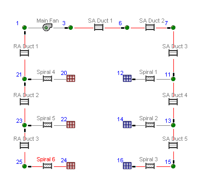
Figure 1. Supply Return system
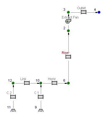
Figure 2. Kitchen Extract
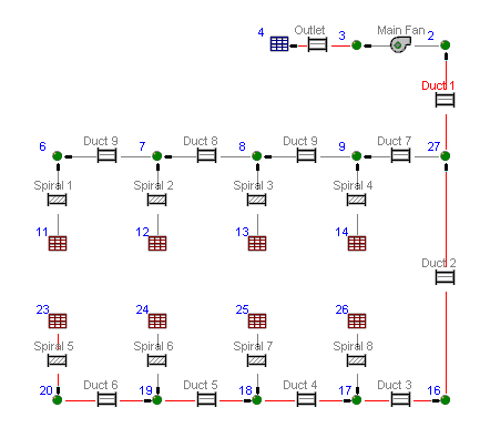
Figure 3. Toilet Extract
SAIRAC 2004 Technical Data Manual, Wernick B.J. Ed.
ASHRAE 2001 Fundamentals Handbook, Duct Design, Chapter 34, pp 33.5
Stoecker, W.F. and Jones, J.W. "Refrigeration & Air Conditioning", 2nd Ed. McGraw Hill 1982.
Massey, B.S. "Mechanics of Fluids", 4th Ed. Von Nostrand Reinhold, 1979.
Moody, L.F. "Friction factors for pipe flow", Transactions of the American Society of Mechanical Engineers, Vol 66 671-684 (1944).
Copyright TechniSolve Software © 2005 All rights reserved
For more information and software, visit the web site